Spiral Matrix III
MediumYou start at the cell (rStart, cStart) of an rows x cols grid facing east. The northwest corner is at the first row and column in the grid, and the southeast corner is at the last row and column.
You will walk in a clockwise spiral shape to visit every position in this grid. Whenever you move outside the grid's boundary, we continue our walk outside the grid (but may return to the grid boundary later.). Eventually, we reach all rows * cols spaces of the grid.
Return an array of coordinates representing the positions of the grid in the order you visited them.
Example 1:
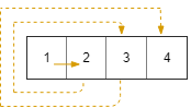
Input: rows = 1, cols = 4, rStart = 0, cStart = 0
Output: [[0,0],[0,1],[0,2],[0,3]]
Example 2:
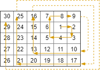
Input: rows = 5, cols = 6, rStart = 1, cStart = 4
Output: [[1,4],[1,5],[2,5],[2,4],[2,3],[1,3],[0,3],[0,4],[0,5],[3,5],[3,4],[3,3],[3,2],[2,2],[1,2],[0,2],[4,5],[4,4],[4,3],[4,2],[4,1],[3,1],[2,1],[1,1],[0,1],[4,0],[3,0],[2,0],[1,0],[0,0]]
Constraints:
1 <= rows, cols <= 1000 <= rStart < rows0 <= cStart < cols
Solution
Clarifying Questions
When you get asked this question in a real-life environment, it will often be ambiguous (especially at FAANG). Make sure to ask these questions in that case:
- Are the row and column indices (r0, c0) guaranteed to be within the bounds of the rows and cols dimensions?
- What should I return if the entire spiral path does not fall within the bounds of the rows and cols dimensions? Should I return only the coordinates that are within bounds?
- Can rows and cols be zero? If so, what is the expected output?
- Are rows and cols guaranteed to be positive integers?
- Is the order of coordinates in the output important? Should they be ordered based on the spiral traversal?
Brute Force Solution
Approach
The brute force approach to traversing a spiral matrix involves simulating the spiral path, step by step. We essentially walk the spiral and record the cells we visit, checking if those cells fall within the matrix boundaries. We continue until we have found the desired number of cells within the boundaries.
Here's how the algorithm would work step-by-step:
- Start at the given starting cell within the matrix.
- Move to the right one step.
- Check if the new cell is within the matrix boundaries. If it is, record it.
- Continue moving right until the number of steps matching the current direction's length have been taken.
- Now, move down two steps.
- Check if the new cell is within the matrix boundaries. If it is, record it.
- Continue moving down until the number of steps matching the current direction's length have been taken.
- Now, move left two steps.
- Check if the new cell is within the matrix boundaries. If it is, record it.
- Continue moving left until the number of steps matching the current direction's length have been taken.
- Now, move up three steps.
- Check if the new cell is within the matrix boundaries. If it is, record it.
- Continue moving up until the number of steps matching the current direction's length have been taken.
- Continue increasing the step counts (3, 4, 4, 5, 5, etc.) and changing directions (right, down, left, up) to simulate the spiral path, and checking if each cell is within bounds, until you've recorded the desired number of valid cells.
Code Implementation
def spiral_matrix_iii(rows, columns, start_row, start_column):    all_coordinates = []
    current_row = start_row
    current_column = start_column
    all_coordinates.append([current_row, current_column])

    # Initialize the step size and the direction
    step_size = 1
    directions = [[0, 1], [1, 0], [0, -1], [-1, 0]]
    direction_index = 0

    # Continue until we have the desired number of coordinates
    while len(all_coordinates) < rows * columns:
        # Move in the current direction for the current step size
        for _ in range(step_size):
            current_row += directions[direction_index][0]
            current_column += directions[direction_index][1]

            # Check if the new coordinate is within bounds
            if 0 <= current_row < rows and 0 <= current_column < columns:
                all_coordinates.append([current_row, current_column])

        # Change direction and increment step size
        direction_index = (direction_index + 1) % 4

        # Increase step size after two directions (right, down, left, up)
        if direction_index % 2 == 0:
            step_size += 1

return all_coordinatesBig(O) Analysis
Optimal Solution
Approach
Instead of exploring the entire matrix randomly, the optimal approach builds the spiral path step-by-step, moving in a specific pattern (right, down, left, up). We extend each direction's movement length after every two directions, ensuring we cover the whole matrix efficiently. We check if the current cell is within the matrix boundaries at each step and add it to the output if it is.
Here's how the algorithm would work step-by-step:
- Begin at the designated starting cell within the matrix.
- Initially, move one step to the right.
- After moving to the right, switch directions and move one step downwards.
- Then, move two steps to the left, extending the movement length.
- Next, move two steps upwards, maintaining the extended movement length.
- Continue this pattern, increasing the number of steps in each direction (right, down, left, up) every two direction changes.
- At each step, check if the new cell's coordinates are within the matrix boundaries.
- If the cell is within the matrix, record its coordinates.
- Continue the spiral pattern until a specified number of cells have been visited.
Code Implementation
def spiral_matrix_iii(rows, columns, start_row, start_column):
    result = []
    row = start_row
    column = start_column
    result.append([row, column])
    if rows * columns == 1:
        return result

    step_length = 1
    # Directions: right, down, left, up
    directions = [[0, 1], [1, 0], [0, -1], [-1, 0]]
    direction_index = 0

    while len(result) < rows * columns:
        # We move in each direction
        for _ in range(2):
            for _ in range(step_length):
                row += directions[direction_index][0]
                column += directions[direction_index][1]

                # Check if the current cell is within the matrix bounds
                if 0 <= row < rows and 0 <= column < columns:
                    result.append([row, column])

                if len(result) == rows * columns:
                    return result

            # Change to the next direction
            direction_index = (direction_index + 1) % 4

            # Increase the step length after two directions
        step_length += 1

return resultBig(O) Analysis
Edge Cases
| Case | How to Handle |
|---|---|
| rows or cols is zero or negative | Return an empty list since the matrix dimensions are invalid. |
| r_start or c_start are outside the bounds of the matrix | Adjust r_start and c_start to be within the valid range of rows and cols respectively; use 0 as the minimum value and rows-1 or cols-1 as the maximum. |
| rows and cols are both 1 | Return a list containing only the starting coordinates since that is the entire matrix. |
| The starting point is close to the edge, causing the spiral to hit the boundary quickly | The algorithm should continue spiraling outwards, even if it means going outside the matrix boundaries, until the desired number of cells is visited. |
| Large rows and cols values leading to many iterations | The algorithm should scale linearly with the number of cells visited (rows * cols) and should not cause stack overflow or excessive memory usage. |
| Rows and cols are different orders of magnitude (e.g., rows = 1, cols = 100) | The spiraling logic must correctly handle drastically different dimensions. |
| The algorithm attempts to access invalid indices outside of the matrix bounds | Implement checks to see if the current coordinates are within the matrix bounds before adding them to the result list. |
| Integer overflow potential when calculating new coordinates | Use long or appropriate data types to prevent integer overflow when calculating coordinates, especially when steps becomes large. |