Cheapest Flights Within K Stops

Medium

Oracle

1 view

Topics:

GraphsDynamic Programming

There are n cities connected by some number of flights. You are given an array flights where flights[i] = [from_i, to_i, price_i] indicates that there is a flight from city from_i to city to_i with cost price_i.

You are also given three integers src, dst, and k, return the cheapest price from src to dst with at most k stops. If there is no such route, return -1.

Example 1:

Input: n = 4, flights = [[0,1,100],[1,2,100],[2,0,100],[1,3,600],[2,3,200]], src = 0, dst = 3, k = 1
Output: 700
Explanation:
The graph is shown above.
The optimal path with at most 1 stop from city 0 to 3 is marked in red and has cost 100 + 600 = 700.
Note that the path through cities [0,1,2,3] is cheaper but is invalid because it uses 2 stops.

Example 2:

Input: n = 3, flights = [[0,1,100],[1,2,100],[0,2,500]], src = 0, dst = 2, k = 1
Output: 200
Explanation:
The graph is shown above.
The optimal path with at most 1 stop from city 0 to 2 is marked in red and has cost 100 + 100 = 200.

Example 3:

Input: n = 3, flights = [[0,1,100],[1,2,100],[0,2,500]], src = 0, dst = 2, k = 0
Output: 500
Explanation:
The graph is shown above.
The optimal path with no stops from city 0 to 2 is marked in red and has cost 500.

Constraints:

1 <= n <= 100
0 <= flights.length <= (n * (n - 1) / 2)
flights[i].length == 3
0 <= from_i, to_i < n
from_i != to_i
1 <= price_i <= 10⁴
There will not be any multiple flights between two cities.
0 <= src, dst, k < n
src != dst

Cheapest Flights Within K Stops

Medium

Oracle

1 view

Topics:

GraphsDynamic Programming

There are n cities connected by some number of flights. You are given an array flights where flights[i] = [from_i, to_i, price_i] indicates that there is a flight from city from_i to city to_i with cost price_i.

You are also given three integers src, dst, and k, return the cheapest price from src to dst with at most k stops. If there is no such route, return -1.

Example 1:

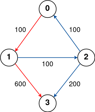
Input: n = 4, flights = [[0,1,100],[1,2,100],[2,0,100],[1,3,600],[2,3,200]], src = 0, dst = 3, k = 1
Output: 700
Explanation:
The graph is shown above.
The optimal path with at most 1 stop from city 0 to 3 is marked in red and has cost 100 + 600 = 700.
Note that the path through cities [0,1,2,3] is cheaper but is invalid because it uses 2 stops.

Example 2:

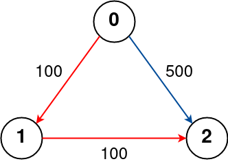
Input: n = 3, flights = [[0,1,100],[1,2,100],[0,2,500]], src = 0, dst = 2, k = 1
Output: 200
Explanation:
The graph is shown above.
The optimal path with at most 1 stop from city 0 to 2 is marked in red and has cost 100 + 100 = 200.

Example 3:

Input: n = 3, flights = [[0,1,100],[1,2,100],[0,2,500]], src = 0, dst = 2, k = 0
Output: 500
Explanation:
The graph is shown above.
The optimal path with no stops from city 0 to 2 is marked in red and has cost 500.

Constraints:

1 <= n <= 100
0 <= flights.length <= (n * (n - 1) / 2)
flights[i].length == 3
0 <= from_i, to_i < n
from_i != to_i
1 <= price_i <= 10⁴
There will not be any multiple flights between two cities.
0 <= src, dst, k < n
src != dst

Solution

Clarifying Questions

When you get asked this question in a real-life environment, it will often be ambiguous (especially at FAANG). Make sure to ask these questions in that case:

What are the constraints on the number of cities `n`, the number of flights, the values of `fromi`, `toi`, `pricei`, `src`, `dst`, and `k`? Are there any upper limits I should be aware of?
Is it possible for there to be cycles in the flight routes?
Is it guaranteed that `src` and `dst` are valid cities (i.e., within the range [0, n-1])?
If there are multiple cheapest paths with at most `k` stops, is any one acceptable, or is there a specific path that should be preferred?
Can the `pricei` be zero or negative?

Brute Force Solution

Approach

We want to find the cheapest flight route from a starting city to a destination city, with a limit on the number of connecting flights. The brute force approach explores every possible flight path to find the cheapest one that meets our requirements.

Here's how the algorithm would work step-by-step:

Start at the departure city.
Consider every flight leaving from that city as a potential first flight.
For each of those first flights, look at all the flights leaving from the city you landed in.
Continue this process, exploring all possible flight combinations, keeping track of the total cost of each route.
Stop exploring a route if it exceeds the maximum number of allowed connecting flights or if the route arrives back at a city already visited (to avoid endless loops).
Once you have explored all possible routes up to the allowed number of connections, compare the total costs of all routes that reached the destination city.
The route with the lowest total cost is your answer.

Code Implementation

def find_cheapest_flights_brute_force(number_of_cities, flights, source, destination, max_stops):
    cheapest_price = float('inf')

    def depth_first_search(current_city, stops_remaining, current_cost, visited):
        nonlocal cheapest_price

        if current_city == destination:
            cheapest_price = min(cheapest_price, current_cost)
            return

        if stops_remaining < 0:
            return

        # Need to check for cycles to avoid infinite recursion
        if current_city in visited:
            return

        visited.add(current_city)

        for start_city, end_city, price in flights:
            if start_city == current_city:
                
                # Explore the next city with reduced stops and increased cost
                depth_first_search(end_city, stops_remaining - 1, current_cost + price, visited.copy())

        visited.remove(current_city)

    # Initialize the depth first search to find the min price
    depth_first_search(source, max_stops, 0, set())

    if cheapest_price == float('inf'):
        return -1
    else:
        return cheapest_price

Try it yourself on LeetCode

Big(O) Analysis

Time Complexity

O(V * (E^(K+1))) – The brute force approach explores all possible paths with at most K stops. In the worst case, from each city, we could potentially explore every edge. This creates a branching factor of E (number of edges) at each level of the search tree. Since we can have at most K intermediate stops, the depth of the search tree is K+1. In the worst-case, we might visit each vertex at each level of our search, leading to a time complexity proportional to V * (E^(K+1)), where V is the number of vertices and E is the number of edges. We multiply by V since, in each layer, the algorithm might consider all possible starting vertices.

Space Complexity

O(N^K) – The algorithm explores all possible flight paths up to K stops. In the worst-case scenario, from each city, we might have to explore flights to nearly every other city. This branching factor leads to an exponential growth of paths explored as we increase the number of stops. The recursion stack can grow to a depth of K, and at each level, we store N possible cities, where N is the number of cities. Keeping track of visited cities to avoid cycles requires space proportional to the length of the path being explored, contributing up to O(K) in each recursive call. Therefore, the overall space complexity is dominated by the potential exploration of N^K paths, leading to an auxiliary space usage of O(N^K).

Optimal Solution

Approach

To find the cheapest flight with a limited number of stops, we explore possible routes step-by-step, always tracking the lowest price we've found so far for each city after a certain number of stops. We use this information to intelligently discard routes that are already more expensive than known cheaper options.

Here's how the algorithm would work step-by-step:

Start at the origin city with a cost of zero.
For each possible number of stops, from zero up to the maximum allowed:
Go through all available flights, considering only flights that depart from cities we reached in the previous round of stops.
For each flight, calculate the total cost to reach the destination city via this flight.
If the total cost is lower than the cheapest price we've previously found to reach that destination city with the current number of stops, update the cheapest price.
After considering all flights for a specific number of stops, move on to the next number of stops.
After exploring all possible routes within the allowed number of stops, the cheapest price recorded for the destination city is the answer. If no route was found, the answer is -1.

Code Implementation

def find_cheapest_price(number_of_cities, flights, source_city, destination_city, max_stops):
    cheapest_prices = {}
    cheapest_prices[source_city] = 0
    
    for current_stop in range(max_stops + 1):
        temp_cheapest_prices = cheapest_prices.copy()
        
        for start_city, end_city, price in flights:
            if start_city in cheapest_prices:
                # Only process flights departing from reached cities.
                current_price = cheapest_prices[start_city] + price

                if end_city not in temp_cheapest_prices or current_price < temp_cheapest_prices[end_city]:
                    # Found a cheaper route to the destination.
                    temp_cheapest_prices[end_city] = current_price
        
        cheapest_prices = temp_cheapest_prices
    
    # Return the cheapest price if found.
    if destination_city in cheapest_prices:
        return cheapest_prices[destination_city]
    else:
        return -1

Try it yourself on LeetCode

Big(O) Analysis

Time Complexity

O(K * |E|) – The algorithm iterates through the number of stops from 0 to K. In each iteration, it examines all the edges (flights) in the graph, represented by |E|, to update the cost to reach each city. Since the algorithm processes all edges for each possible number of stops, the total time complexity is proportional to the product of K and the number of edges |E|. Therefore, the overall time complexity is O(K * |E|).

Space Complexity

O(N) – The algorithm uses a data structure to store the cheapest price found so far for each city after a certain number of stops. This data structure effectively stores the minimum cost to reach each city for each stop, which will have a size proportional to the number of cities multiplied by the number of stops considered. Since the maximum number of stops is K, and assuming we have N cities, we need to keep track of the minimum cost to reach each of the N cities for each stop up to K, or in the worst-case, up to N stops, therefore this cheapest price information will grow in proportion to N. Consequently, the auxiliary space used is O(N).

Edge Cases

Case	How to Handle
flights is null or empty	If flights is null or empty, and src != dst return -1, else if flights is null or empty and src == dst return 0.
n is zero or negative	If n is non-positive, there can be no valid path, return -1.
k is negative	If k is negative, it is an invalid input, return -1.
src is equal to dst	If src is equal to dst, the cost is 0 regardless of the number of stops, so return 0.
No path exists from src to dst within k stops	If after exploring all possible paths within k stops, dst is not reached, return -1.
Integer overflow during price calculation	Use long data type to store prices during calculation and before returning, or check if the running total exceeds a maximum amount (like Integer.MAX_VALUE).
Graph contains cycles	The BFS/Bellman-Ford algorithm naturally handles cycles by tracking the number of stops/iterations and ensuring it doesn't exceed k.
Maximum values for n, k and prices that could lead to TLE (Time Limit Exceeded)	Optimize the algorithm to use Dijkstra or Bellman-Ford with efficient priority queue or early stopping conditions to avoid unnecessary computations.