Maximal Square
MediumGiven an m x n binary matrix filled with 0's and 1's, find the largest square containing only 1's and return its area.
Example 1:
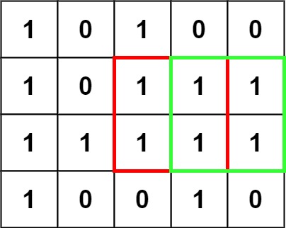
Input: matrix = [["1","0","1","0","0"],["1","0","1","1","1"],["1","1","1","1","1"],["1","0","0","1","0"]]
Output: 4
Example 2:

Input: matrix = [["0","1"],["1","0"]]
Output: 1
Example 3:
Input: matrix = [["0"]]
Output: 0
Constraints:
m == matrix.lengthn == matrix[i].length1 <= m, n <= 300matrix[i][j]is'0'or'1'.
Solution
Clarifying Questions
When you get asked this question in a real-life environment, it will often be ambiguous (especially at FAANG). Make sure to ask these questions in that case:
- What are the dimensions of the matrix (rows and columns), and are there any constraints on their sizes? Can either dimension be zero or empty?
- Is the input matrix guaranteed to contain only '0' and '1' characters, or could there be other characters present?
- If the matrix contains no '1's (i.e., only '0's), what should the function return? Should it return 0, or should an exception be raised?
- Is the input matrix always rectangular (i.e., all rows have the same number of columns)?
- By 'area', do you specifically mean the side length of the largest square squared, or should I return the side length itself?
Brute Force Solution
Approach
The brute force approach to finding the biggest square of ones in a grid involves checking every possible square, one by one. We systematically look at all potential square sizes and starting positions within the grid to see if they are valid squares composed entirely of ones.
Here's how the algorithm would work step-by-step:
- Consider every possible location in the grid as the top-left corner of a potential square.
- For each of these locations, try to form squares of increasing sizes, starting with size 1.
- For each square size, carefully examine all the cells within that square to see if they all contain the value '1'.
- If even a single cell within the square contains a '0', then that square is invalid, and we discard it.
- If all cells within the square contain '1', then we have found a valid square.
- Keep track of the size of the largest valid square we have found so far.
- Continue checking all possible locations and square sizes, updating the largest valid square size whenever a larger one is found.
- Once we have checked all possible locations and sizes, the size of the largest valid square we tracked is the answer.
Code Implementation
def maximal_square_brute_force(matrix):
    if not matrix:
        return 0

    rows = len(matrix)
    cols = len(matrix[0])
    max_side = 0

    for row_index in range(rows):
        for col_index in range(cols):
            # Consider each cell as top-left
            for side_length in range(1, min(rows - row_index, cols - col_index) + 1):
                is_square = True

                # Check if all cells are '1'
                for i in range(row_index, row_index + side_length):

                    for j in range(col_index, col_index + side_length):
                        if matrix[i][j] == '0':
                            is_square = False
                            break
                    if not is_square:
                        break

                # Update max_side if valid
                if is_square:

                    max_side = max(max_side, side_length)

return max_side * max_sideBig(O) Analysis
Optimal Solution
Approach
The goal is to find the biggest square made of only 1s within a grid of 0s and 1s. Instead of checking every possible square size at every location, we use a technique to build up square sizes incrementally.
Here's how the algorithm would work step-by-step:
- Imagine each cell in the grid represents the bottom-right corner of a potential square.
- Start by considering the current cell. If it's a 0, then it can't be part of any square, so the size of the biggest square ending there is 0.
- If the current cell is a 1, then the biggest square ending there is at least of size 1 (just the cell itself).
- Now, to see if we can make a bigger square, look at the cells directly to the left, directly above, and diagonally above and to the left of the current cell.
- The size of the biggest square ending at the current cell is one more than the SMALLEST of the sizes of the squares ending at those three neighboring cells.
- For example, if those three neighboring squares have sizes 1, 2, and 1, then the biggest square ending at the current cell is of size 2 (1+1). The current square can only be as big as its weakest neighbor allows.
- Keep track of the biggest square size you find throughout the entire grid. This will be the answer.
- By working through the grid in this way, you only calculate the size of the biggest possible square at each location, instead of trying out all the possible sizes.
Code Implementation
def maximal_square(matrix):
    number_of_rows = len(matrix)
    number_of_columns = len(matrix[0]) if number_of_rows > 0 else 0
    size_of_largest_square = 0
    # This table stores max square size ending at each cell.
    square_sizes = [[0] * number_of_columns for _ in range(number_of_rows)]

    for row_index in range(number_of_rows):
        for column_index in range(number_of_columns):
            if matrix[row_index][column_index] == '1':
                # Base case: single cell is a square of size 1.
                square_sizes[row_index][column_index] = 1

                if row_index > 0 and column_index > 0:
                    # Find minimum size of neighbors to expand square.
                    square_sizes[row_index][column_index] = min(
                        square_sizes[row_index-1][column_index],
                        square_sizes[row_index][column_index-1],
                        square_sizes[row_index-1][column_index-1]
                    ) + 1

                # Track the largest square found.
                size_of_largest_square = max(
                    size_of_largest_square,
                    square_sizes[row_index][column_index]
                )

    # Return area, which is the side length squared.
return size_of_largest_square * size_of_largest_squareBig(O) Analysis
Edge Cases
| Case | How to Handle |
|---|---|
| Null or empty matrix | Return 0 immediately since no square can exist. |
| Matrix with zero rows or columns | Return 0 immediately as an empty matrix has no area. |
| Matrix with a single row and single column containing a 1 | Return 1 because a 1x1 square exists. |
| Matrix with a single row or column containing only 0s | Return 0 because no square of 1s exists. |
| Matrix filled entirely with 0s | Return 0, as the largest square will have side length 0. |
| Matrix filled entirely with 1s | Return the area of the entire matrix, which is a square with side min(rows, cols). |
| Large matrix where the largest square is located in the bottom right corner. | The dynamic programming approach will correctly propagate the square size information from top-left to bottom-right. |
| Integer overflow when calculating the area for very large matrices | Ensure intermediate area calculations use a larger data type (e.g., long) or consider returning the side length squared. |