Count Number of Possible Root Nodes
HardAlice has an undirected tree with n nodes labeled from 0 to n - 1. The tree is represented as a 2D integer array edges of length n - 1 where edges[i] = [ai, bi] indicates that there is an edge between nodes ai and bi in the tree.
Alice wants Bob to find the root of the tree. She allows Bob to make several guesses about her tree. In one guess, he does the following:
- Chooses two distinct integers
uandvsuch that there exists an edge[u, v]in the tree. - He tells Alice that
uis the parent ofvin the tree.
Bob's guesses are represented by a 2D integer array guesses where guesses[j] = [uj, vj] indicates Bob guessed uj to be the parent of vj.
Alice being lazy, does not reply to each of Bob's guesses, but just says that at least k of his guesses are true.
Given the 2D integer arrays edges, guesses and the integer k, return the number of possible nodes that can be the root of Alice's tree. If there is no such tree, return 0.
Example 1:
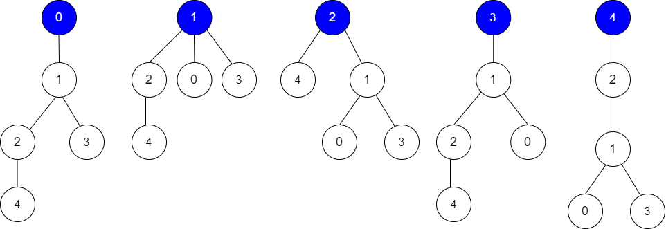
Input: edges = [[0,1],[1,2],[1,3],[4,2]], guesses = [[1,3],[0,1],[1,0],[2,4]], k = 3
Output: 3
Explanation:
Root = 0, correct guesses = [1,3], [0,1], [2,4]
Root = 1, correct guesses = [1,3], [1,0], [2,4]
Root = 2, correct guesses = [1,3], [1,0], [2,4]
Root = 3, correct guesses = [1,0], [2,4]
Root = 4, correct guesses = [1,3], [1,0]
Considering 0, 1, or 2 as root node leads to 3 correct guesses.
Example 2:
Input: edges = [[0,1],[1,2],[2,3],[3,4]], guesses = [[1,0],[3,4],[2,1],[3,2]], k = 1
Output: 5
Explanation:
Root = 0, correct guesses = [3,4]
Root = 1, correct guesses = [1,0], [3,4]
Root = 2, correct guesses = [1,0], [2,1], [3,4]
Root = 3, correct guesses = [1,0], [2,1], [3,2], [3,4]
Root = 4, correct guesses = [1,0], [2,1], [3,2]
Considering any node as root will give at least 1 correct guess.
Constraints:
edges.length == n - 12 <= n <= 1051 <= guesses.length <= 1050 <= ai, bi, uj, vj <= n - 1ai != biuj != vjedgesrepresents a valid tree.guesses[j]is an edge of the tree.guessesis unique.0 <= k <= guesses.length
Solution
Clarifying Questions
When you get asked this question in a real-life environment, it will often be ambiguous (especially at FAANG). Make sure to ask these questions in that case:
- What are the constraints on the range of values within the nodes and edges?
- Can the graph represented by the edges be disconnected?
- Is it guaranteed that the input 'edges' represents a valid tree structure (no cycles, etc.)?
- If there are no possible root nodes satisfying the condition, what should the function return?
- Are the 'guesses' guaranteed to be valid edges existing in the 'edges' input?
Brute Force Solution
Approach
The brute force approach systematically tests every single node as a potential root to see if it satisfies the given constraints. For each possible root, we'll verify whether the provided relationships hold true. This exhaustive method guarantees finding the correct count, but it can be quite slow.
Here's how the algorithm would work step-by-step:
- Pick any node from the entire set of nodes and temporarily designate it as the 'root' of the tree.
- Using this chosen root, go through each relationship to check if the relationship aligns with this 'root' choice. We must be able to determine the relationship between nodes based on the proposed root.
- If even one relationship doesn't hold true based on the chosen root, then this node cannot be the correct root.
- If all the relationships hold true with the selected root, increment a counter that tracks the number of valid roots.
- Repeat the process by selecting a different node from the set of nodes as the potential root.
- Continue this process until every node has been tested as a potential root.
- The final count represents the number of nodes that could validly serve as the root of the tree based on the provided relationships.
Code Implementation
def count_possible_root_nodes_brute_force(number_of_nodes, edges, guesses):
    valid_root_count = 0

    for potential_root in range(number_of_nodes):
        is_valid_root = True

        # Iterate through each guess to validate the potential root.
        for parent, child in guesses:
            is_correct_guess = False

            # Perform a depth first search to determine the relationship.
            def depth_first_search(start_node, target_node, current_path):
                if start_node == target_node:
                    return True

                for neighbor in get_neighbors(start_node, edges):
                    if neighbor not in current_path:
                        if depth_first_search(neighbor, target_node, current_path + [neighbor]):
                            return True
                return False

            # Check if parent is actually an ancestor of child.
            if depth_first_search(potential_root, parent, [potential_root]) and depth_first_search(parent, child, [parent]):
                is_correct_guess = True

            if not is_correct_guess:
                is_valid_root = False
                break

        # Increment the count if all guesses were correct for the root.
        if is_valid_root:
            valid_root_count += 1

    return valid_root_count

def get_neighbors(node, edges):
    neighbors = []
    for parent, child in edges:
        if parent == node:
            neighbors.append(child)
        if child == node:
            neighbors.append(parent)
return neighborsBig(O) Analysis
Optimal Solution
Approach
The problem asks us to find how many nodes in a tree could be the root, given some observations about parent-child relationships. The key idea is to first assume a node is the root and check how many observations it satisfies. We then use clever math to update the satisfaction count efficiently when we switch the assumed root to a neighboring node.
Here's how the algorithm would work step-by-step:
- Pick any node and pretend it's the root of the tree.
- Go through all the given parent-child observations and count how many of them match with the chosen root.
- Now, pick a neighbor of the current assumed root. We want to quickly figure out how the observation count would change if this neighbor were the root.
- When we switch to the neighbor as the root, some parent-child observations will now be correct that weren't before, and some will become incorrect. We can figure out exactly which observations flip their correctness.
- Update the count of correct observations based on the changes that happened by switching the root to the neighbor.
- Repeat this process for all nodes in the tree, always starting from the initial root and moving to its neighbors, and then to their neighbors, and so on.
- Keep track of the observation count for each node when it's assumed to be the root.
- Finally, go through all the observation counts. The number of nodes that have an observation count equal to the total number of provided observations is the answer.
Code Implementation
def count_valid_root_nodes(number_of_nodes, edges, guesses):
    graph = [[] for _ in range(number_of_nodes)]
    for u, v in edges:
        graph[u].append(v)
        graph[v].append(u)

    def calculate_initial_score(root_node):
        score = 0
        for parent, child in guesses:
            if is_parent_child(root_node, parent, child):
                score += 1
        return score

    def is_parent_child(root_node, parent, child):
        if parent == root_node:
            return False

        queue = [root_node]
        visited = {root_node}

        while queue:
            node = queue.pop(0)
            if node == parent:
                queue2 = [root_node]
                visited2 = {root_node}
                while queue2:
                    node2 = queue2.pop(0)
                    if node2 == child:
                        return False
                    for neighbor in graph[node2]:
                        if neighbor not in visited2:
                            visited2.add(neighbor)
                            queue2.append(neighbor)
                return True

            for neighbor in graph[node]:
                if neighbor not in visited:
                    visited.add(neighbor)
                    queue.append(neighbor)

        return False

    node_scores = [0] * number_of_nodes
    node_scores[0] = calculate_initial_score(0)

    # Use DFS to propagate the score from the initial root
    def dfs(current_node, parent_node):
        for neighbor in graph[current_node]:
            if neighbor != parent_node:
                # Efficiently update the score based on guess changes
                node_scores[neighbor] = node_scores[current_node]
                for parent, child in guesses:
                    if (is_parent_child(current_node, parent, child) and not is_parent_child(neighbor, parent, child)):
                        node_scores[neighbor] -= 1
                    elif (not is_parent_child(current_node, parent, child) and is_parent_child(neighbor, parent, child)):
                        node_scores[neighbor] += 1
                dfs(neighbor, current_node)

    dfs(0, -1)

    # Count nodes that have a perfect score
    count = 0
    for score in node_scores:
        if score == len(guesses):
            count += 1

return countBig(O) Analysis
Edge Cases
| Case | How to Handle |
|---|---|
| Empty edges array and guesses array | Return 0 as there are no edges or guesses to evaluate. |
| Empty edges array, non-empty guesses array | Return 0, since no real root can be inferred when no edges exist. |
| Empty guesses array, non-empty edges array | The true root is simply the number of nodes with in-degree matching the number of edges, initialize count with that and return. |
| Edges form a cycle | The problem doesn't explicitly state that the graph must be a tree, so the solution must correctly handle cycles (e.g., through careful traversal or by ignoring back edges). |
| Guesses that are not valid edges | The solution should only consider guesses which exist as edges when calculating the possible roots. |
| Large number of nodes and edges | Use efficient data structures (e.g., hash maps) for adjacency lists and edge lookups to maintain reasonable time complexity O(E) where E is the number of edges. |
| Graph is disconnected | Ensure the traversal covers all connected components to accurately count root possibilities. |
| All guesses are correct | The chosen root will match all guesses and should be counted towards the final result. |