Minimum Cost to Reach Destination in Time

Hard

Asked by:

8 views

Topics:

GraphsDynamic Programming

There is a country of n cities numbered from 0 to n - 1 where all the cities are connected by bi-directional roads. The roads are represented as a 2D integer array edges where edges[i] = [x_i, y_i, time_i] denotes a road between cities x_i and y_i that takes time_i minutes to travel. There may be multiple roads of differing travel times connecting the same two cities, but no road connects a city to itself.

Each time you pass through a city, you must pay a passing fee. This is represented as a 0-indexed integer array passingFees of length n where passingFees[j] is the amount of dollars you must pay when you pass through city j.

In the beginning, you are at city 0 and want to reach city n - 1 in maxTime minutes or less. The cost of your journey is the summation of passing fees for each city that you passed through at some moment of your journey (including the source and destination cities).

Given maxTime, edges, and passingFees, return the minimum cost to complete your journey, or -1 if you cannot complete it within maxTime minutes.

Example 1:

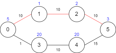
Input: maxTime = 30, edges = [[0,1,10],[1,2,10],[2,5,10],[0,3,1],[3,4,10],[4,5,15]], passingFees = [5,1,2,20,20,3]
Output: 11
Explanation: The path to take is 0 -> 1 -> 2 -> 5, which takes 30 minutes and has $11 worth of passing fees.

Example 2:

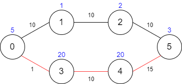
Input: maxTime = 29, edges = [[0,1,10],[1,2,10],[2,5,10],[0,3,1],[3,4,10],[4,5,15]], passingFees = [5,1,2,20,20,3]
Output: 48
Explanation: The path to take is 0 -> 3 -> 4 -> 5, which takes 26 minutes and has $48 worth of passing fees.
You cannot take path 0 -> 1 -> 2 -> 5 since it would take too long.

Example 3:

Input: maxTime = 25, edges = [[0,1,10],[1,2,10],[2,5,10],[0,3,1],[3,4,10],[4,5,15]], passingFees = [5,1,2,20,20,3]
Output: -1
Explanation: There is no way to reach city 5 from city 0 within 25 minutes.

Constraints:

1 <= maxTime <= 1000
n == passingFees.length
2 <= n <= 1000
n - 1 <= edges.length <= 1000
0 <= x_i, y_i <= n - 1
1 <= time_i <= 1000
1 <= passingFees[j] <= 1000
The graph may contain multiple edges between two nodes.
The graph does not contain self loops.

Try coding it in LeetCode

Solution

Clarifying Questions

When you get asked this question in a real-life environment, it will often be ambiguous (especially at FAANG). Make sure to ask these questions in that case:

What are the maximum values for `maxTime`, `passingFees` array elements, and the number of cities `n`? This will help me understand potential overflow issues and the scale of the problem.
Can the `passingFees` array contain zero or negative values? Is it guaranteed that the starting and ending cities have non-negative fees?
Is it possible to have a scenario where it's impossible to reach the destination within `maxTime`? If so, what value should I return in that case?
Are the paths between cities directed or undirected? If directed, is there any guarantee about the presence or absence of cycles?
Can there be multiple paths between two cities? If so, should I consider the fastest path between any two cities in my time calculation, or should I treat each path as a distinct edge in a graph?

Brute Force Solution

Approach

The core idea is to explore absolutely every possible path from the starting point to the destination. We calculate the cost of each path and eliminate those that don't meet the time limit. Finally, we choose the path with the lowest cost from all possible valid paths.

Here's how the algorithm would work step-by-step:

Start at the beginning point.
Consider all possible routes we can take from our current location to the next possible location.
For each of these routes, calculate the total time it would take to reach the destination, and the total cost (or fuel) it would require.
If a route takes longer than the allowed time, we throw that route away and don't consider it further.
If a route reaches the destination within the allowed time, we save its total cost.
Repeat steps 2-5 for every possible sequence of routes until all options have been considered.
Once we have explored all possible routes and their costs, find the route with the lowest cost from all routes that met the time constraint. That's our answer.

Code Implementation

def minimum_cost_to_reach_destination_brute_force(max_time, passing_fees, time_costs):
    number_of_cities = len(passing_fees)
    minimum_possible_cost = float('inf')

    def explore_all_paths(current_city, current_time, current_cost):
        nonlocal minimum_possible_cost

        # If time exceeds max_time, stop
        if current_time > max_time:
            return

        # If reached the destination
        if current_city == number_of_cities - 1:
            minimum_possible_cost = min(minimum_possible_cost, current_cost + passing_fees[current_city])
            return

        # Explore all possible next cities
        for next_city in range(number_of_cities):
            if next_city != current_city:

                # Ensuring we don't revisit the same city
                time_to_next_city = time_costs[current_city][next_city]

                # Recursive call to explore paths
                explore_all_paths(next_city, current_time + time_to_next_city, current_cost + passing_fees[current_city])

    # Start exploring from city 0 with initial time 0 and cost 0
    explore_all_paths(0, 0, 0)

    # If no path is found within max_time, return -1
    if minimum_possible_cost == float('inf'):
        return -1
    else:
        return minimum_possible_cost

Big(O) Analysis

Time Complexity

O(N!) – The algorithm explores all possible paths from the starting point to the destination, which resembles a brute-force approach. In the worst-case scenario, where the graph is densely connected, the number of possible paths grows factorially with the number of cities (N). This is because at each city, we might have to explore almost all remaining cities as potential next steps. Therefore, the time complexity is dominated by the factorial growth of possible paths, resulting in O(N!).

Space Complexity

O(V^T) – The algorithm explores all possible paths using a recursive approach (or a similar approach like DFS or BFS if implemented iteratively), where V is the number of cities (vertices in a graph representation) and T is the maximum allowed time. The recursion stack (or queue in BFS) can grow up to a depth that depends on the number of cities visited within the time limit. In the worst-case scenario, we might explore all possible combinations of cities within the time limit, leading to an exponential number of paths being stored either implicitly via the call stack or explicitly in a data structure to track paths. Thus, the space complexity is proportional to the number of possible paths, which can be approximated as O(V^T), where V is the number of vertices, and T is the time limit.

Optimal Solution

Approach

The best way to solve this problem is to explore possible paths in a smart order, keeping track of the fastest ways to get somewhere. We can make use of an advanced searching strategy to effectively find the lowest cost to reach the destination within the given time limit.

Here's how the algorithm would work step-by-step:

Think of this problem like finding the cheapest way to travel from one city to another, but with time limits and costs associated with each city.
We'll start at the beginning and consider different routes we can take.
Each time we consider going to a new city, we'll add its cost to our total cost and the time it takes to travel there to our total time.
We only want to go to a city if we can reach it without exceeding our total allowed travel time.
Keep track of the lowest cost it takes to reach each city, so you can remember and compare with other possibilities.
The clever part is to explore the paths that are more promising first. This means prioritizing paths that have low costs and take less time.
As we explore, if we find a better (lower cost) way to get to a city than we previously knew, we update our record.
Continue this process until we have explored all reasonable routes and found the minimum cost to reach our final destination within the time limit.
If we can't reach the final destination within the time limit, we'll report that it's impossible.

Code Implementation

import heapq

def minCost(max_time, city_costs, allowed_travel_times):
    number_of_cities = len(city_costs)
    minimum_costs = [float('inf')] * number_of_cities
    minimum_costs[0] = city_costs[0]

    # Use a priority queue to explore promising paths first.
    priority_queue = [(city_costs[0], 0, 0)]

    while priority_queue:
        current_cost, current_city, current_time = heapq.heappop(priority_queue)

        # If we've exceeded the allowed time, this path is invalid.
        if current_time > max_time:
            continue

        # If we've reached the destination, return the cost
        if current_city == number_of_cities - 1:
            return current_cost

        for next_city, travel_time in enumerate(allowed_travel_times[current_city]):
            if travel_time > 0:
                new_time = current_time + travel_time
                # Prune paths that exceed the time limit
                if new_time <= max_time:

                    new_cost = current_cost + city_costs[next_city]
                    # Update minimum cost if a better path is found
                    if new_cost < minimum_costs[next_city]:

                        minimum_costs[next_city] = new_cost
                        # Add the new state to the priority queue
                        heapq.heappush(priority_queue, (new_cost, next_city, new_time))

    return -1

Big(O) Analysis

Time Complexity

O(T * N * logN) – The algorithm uses a priority queue (heap) to explore paths, where N is the number of cities (nodes) and T is the maximum allowed time. In the worst case, we might explore each city multiple times, potentially up to T times, based on different arrival times at that city. Each time we add a city to the priority queue, it takes O(logN) time to maintain the heap property. Therefore, the overall time complexity is approximately O(T * N * logN) as we might potentially visit each node up to T times and perform logN operations on the priority queue during each visit.

Space Complexity

O(N) – The algorithm uses a data structure to keep track of the lowest cost to reach each city (step 5 and 7). In the worst case, we might need to store the lowest cost for every city. If we have N cities, this would require an auxiliary array or hash map of size N. The priority queue used to explore promising paths first (step 6) can also, in the worst case, contain entries for all N cities. Therefore, the auxiliary space used is proportional to the number of cities, N, leading to a space complexity of O(N).

Edge Cases

Case	How to Handle
Empty `passingFees` or `timeLimits` array, or null input	Return -1 immediately as there's no path or time to calculate the cost.
`n` (number of cities) is 1, but `maxTime` is positive	Return 0 since we're already at the destination with no travel required.
`maxTime` is 0, but `n` is greater than 1	Return -1 because it's impossible to reach the destination in zero time.
A city is unreachable within `maxTime`.	The algorithm should propagate the maximum cost (infinity) and eventually return -1 if the destination remains unreachable.
`passingFees` or `timeLimits` contain negative numbers.	Return -1, since negative fees or travel times are invalid inputs.
`timeLimits` values are very large, potentially leading to integer overflow when summed.	Use `long` data type for time calculations to prevent overflow.
The graph contains cycles and the optimal path uses a cycle	Dijkstra's algorithm with time limit handles cycles by tracking the minimum cost to reach each node within the allowed time, effectively ignoring redundant cycles.
Large input sizes for `n` and number of edges may lead to Time Limit Exceeded (TLE).	Optimize algorithm using priority queue (heap) with Dijkstra or A* search to efficiently explore possible paths.

Empty `passingFees` or `timeLimits` array, or null input

How to Handle:

Return -1 immediately as there's no path or time to calculate the cost.

`n` (number of cities) is 1, but `maxTime` is positive

How to Handle:

Return 0 since we're already at the destination with no travel required.

`maxTime` is 0, but `n` is greater than 1

How to Handle:

Return -1 because it's impossible to reach the destination in zero time.

A city is unreachable within `maxTime`.

How to Handle:

The algorithm should propagate the maximum cost (infinity) and eventually return -1 if the destination remains unreachable.

`passingFees` or `timeLimits` contain negative numbers.

How to Handle:

Return -1, since negative fees or travel times are invalid inputs.

`timeLimits` values are very large, potentially leading to integer overflow when summed.

How to Handle:

Use `long` data type for time calculations to prevent overflow.

The graph contains cycles and the optimal path uses a cycle

How to Handle:

Dijkstra's algorithm with time limit handles cycles by tracking the minimum cost to reach each node within the allowed time, effectively ignoring redundant cycles.

Large input sizes for `n` and number of edges may lead to Time Limit Exceeded (TLE).

How to Handle:

Optimize algorithm using priority queue (heap) with Dijkstra or A* search to efficiently explore possible paths.