Minimum Cost Walk in Weighted Graph

Hard

DE Shaw

0 views

Topics:

Graphs

There is an undirected weighted graph with n vertices labeled from 0 to n - 1.

You are given the integer n and an array edges, where edges[i] = [u_i, v_i, w_i] indicates that there is an edge between vertices u_i and v_i with a weight of w_i.

A walk on a graph is a sequence of vertices and edges. The walk starts and ends with a vertex, and each edge connects the vertex that comes before it and the vertex that comes after it. It's important to note that a walk may visit the same edge or vertex more than once.

The cost of a walk starting at node u and ending at node v is defined as the bitwise AND of the weights of the edges traversed during the walk. In other words, if the sequence of edge weights encountered during the walk is w₀, w₁, w₂, ..., w_k, then the cost is calculated as w₀ & w₁ & w₂ & ... & w_k, where & denotes the bitwise AND operator.

You are also given a 2D array query, where query[i] = [s_i, t_i]. For each query, you need to find the minimum cost of the walk starting at vertex s_i and ending at vertex t_i. If there exists no such walk, the answer is -1.

Return the array answer, where answer[i] denotes the minimum cost of a walk for query i.

Example 1:

Input: n = 5, edges = [[0,1,7],[1,3,7],[1,2,1]], query = [[0,3],[3,4]]

Output: [1,-1]

Explanation:

To achieve the cost of 1 in the first query, we need to move on the following edges: 0->1 (weight 7), 1->2 (weight 1), 2->1 (weight 1), 1->3 (weight 7).

In the second query, there is no walk between nodes 3 and 4, so the answer is -1.

Example 2:

Input: n = 3, edges = [[0,2,7],[0,1,15],[1,2,6],[1,2,1]], query = [[1,2]]

Output: [0]

Explanation:

To achieve the cost of 0 in the first query, we need to move on the following edges: 1->2 (weight 1), 2->1 (weight 6), 1->2 (weight 1).

Constraints:

2 <= n <= 10⁵
0 <= edges.length <= 10⁵
edges[i].length == 3
0 <= u_i, v_i <= n - 1
u_i != v_i
0 <= w_i <= 10⁵
1 <= query.length <= 10⁵
query[i].length == 2
0 <= s_i, t_i <= n - 1
s_i != t_i

Minimum Cost Walk in Weighted Graph

Hard

DE Shaw

0 views

Topics:

Graphs

There is an undirected weighted graph with n vertices labeled from 0 to n - 1.

You are given the integer n and an array edges, where edges[i] = [u_i, v_i, w_i] indicates that there is an edge between vertices u_i and v_i with a weight of w_i.

A walk on a graph is a sequence of vertices and edges. The walk starts and ends with a vertex, and each edge connects the vertex that comes before it and the vertex that comes after it. It's important to note that a walk may visit the same edge or vertex more than once.

The cost of a walk starting at node u and ending at node v is defined as the bitwise AND of the weights of the edges traversed during the walk. In other words, if the sequence of edge weights encountered during the walk is w₀, w₁, w₂, ..., w_k, then the cost is calculated as w₀ & w₁ & w₂ & ... & w_k, where & denotes the bitwise AND operator.

You are also given a 2D array query, where query[i] = [s_i, t_i]. For each query, you need to find the minimum cost of the walk starting at vertex s_i and ending at vertex t_i. If there exists no such walk, the answer is -1.

Return the array answer, where answer[i] denotes the minimum cost of a walk for query i.

Example 1:

Input: n = 5, edges = [[0,1,7],[1,3,7],[1,2,1]], query = [[0,3],[3,4]]

Output: [1,-1]

Explanation:

To achieve the cost of 1 in the first query, we need to move on the following edges: 0->1 (weight 7), 1->2 (weight 1), 2->1 (weight 1), 1->3 (weight 7).

In the second query, there is no walk between nodes 3 and 4, so the answer is -1.

Example 2:

Input: n = 3, edges = [[0,2,7],[0,1,15],[1,2,6],[1,2,1]], query = [[1,2]]

Output: [0]

Explanation:

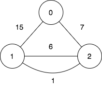
To achieve the cost of 0 in the first query, we need to move on the following edges: 1->2 (weight 1), 2->1 (weight 6), 1->2 (weight 1).

Constraints:

2 <= n <= 10⁵
0 <= edges.length <= 10⁵
edges[i].length == 3
0 <= u_i, v_i <= n - 1
u_i != v_i
0 <= w_i <= 10⁵
1 <= query.length <= 10⁵
query[i].length == 2
0 <= s_i, t_i <= n - 1
s_i != t_i

Solution

Clarifying Questions

When you get asked this question in a real-life environment, it will often be ambiguous (especially at FAANG). Make sure to ask these questions in that case:

What are the constraints on the number of nodes and edges in the graph? Can I assume they fit in memory?
Are the edge weights guaranteed to be non-negative integers?
Is the graph directed or undirected?
If there is no path between the start and end nodes, what should I return? (e.g., -1, infinity, null)
Is the graph guaranteed to be connected?

Brute Force Solution

Approach

The brute force approach to finding the cheapest path involves trying every possible route from the start to the end. We explore all paths regardless of how long or expensive they might seem initially. Eventually, we can compare all the paths and pick the one with the lowest total cost.

Here's how the algorithm would work step-by-step:

Start at the beginning point.
Consider all the possible places you can go directly from the beginning.
For each of those places, consider all the places you can go from there.
Continue this process, building up all possible routes, until you reach the destination.
Keep track of the total cost of each route as you build it.
Once you've explored all possible routes to the destination, compare the total costs.
The route with the smallest total cost is the cheapest path.

Code Implementation

def minimum_cost_walk_brute_force(graph, start_node, end_node):
    def find_all_paths(current_node, current_path, current_cost):
        # If we've reached the end node, add the path to the list of paths.
        if current_node == end_node:
            all_paths.append((current_path, current_cost))
            return

        # Explore all neighbors of the current node.
        for neighbor, cost in graph[current_node].items():
            find_all_paths(neighbor, current_path + [neighbor], current_cost + cost)

    all_paths = []
    find_all_paths(start_node, [start_node], 0)

    # Handle case where no paths exist
    if not all_paths:
        return None

    # Find the path with the minimum cost.
    minimum_cost = float('inf')
    cheapest_path = None

    for path, cost in all_paths:
        if cost < minimum_cost:
            # Update the minimum cost and cheapest path found.
            minimum_cost = cost
            cheapest_path = path

    return cheapest_path

Try it yourself on LeetCode

Big(O) Analysis

Time Complexity

O(V^V) – The brute force approach explores every possible path in the graph. In the worst-case scenario, the algorithm could visit every vertex (V) in the graph multiple times, potentially creating paths of length V. Since we are checking all possible routes and, for each vertex, considering all possible subsequent vertices, the number of possible paths grows exponentially with the number of vertices. Therefore, the time complexity is O(V^V) reflecting the maximum possible paths.

Space Complexity

O(V^V) – The brute force approach explores all possible paths, which can lead to exponential space complexity. In the worst-case scenario, where V is the number of vertices, we might have to store all possible paths of length up to V. The number of such paths can grow as V^V as we are essentially exploring all possible sequences of vertices, resulting in temporary lists to hold each path being explored. Therefore, the space complexity is approximately O(V^V), to store all possible paths.

Optimal Solution

Approach

The best way to find the cheapest path through a graph is to explore paths in order of increasing cost, always keeping track of the shortest distance found so far to each location. This ensures that when we reach the final destination, we have definitely found the minimum cost path. It's like constantly updating the 'best route' on a map as you explore different options.

Here's how the algorithm would work step-by-step:

Start at the beginning point and assign it a cost of zero.
Consider all the places you can directly reach from your current location.
Calculate the total cost to reach each of these places from the start (the cost to get to your current location plus the cost to go to the new place).
Keep track of the shortest cost to get to each location you've visited so far. If you find a cheaper way to get to a place you've already visited, update the shortest cost.
Now, pick the unvisited place that has the smallest cost to reach from the starting point.
Repeat steps 2-5, considering all places reachable from this new location, until you reach your final destination.
The cost you have recorded for the final destination is the minimum cost to get there from the beginning.

Code Implementation

import heapq

def find_minimum_cost_walk(graph, start_node, end_node):
    number_of_nodes = len(graph)
    shortest_distances = {node: float('inf') for node in range(number_of_nodes)}
    shortest_distances[start_node] = 0

    priority_queue = [(0, start_node)]

    while priority_queue:
        current_distance, current_node = heapq.heappop(priority_queue)

        # If we've found a shorter path, skip
        if current_distance > shortest_distances[current_node]:
            continue

        # Iterate through neighbors and find shorter paths
        for neighbor, weight in graph[current_node]:
            distance = current_distance + weight

            # If a shorter path is found, update shortest_distances
            if distance < shortest_distances[neighbor]:
                shortest_distances[neighbor] = distance
                heapq.heappush(priority_queue, (distance, neighbor))

    # Return the minimum cost to reach the end node
    return shortest_distances[end_node]

Try it yourself on LeetCode

Big(O) Analysis

Time Complexity

O(E log V) – The algorithm uses Dijkstra's algorithm to find the minimum cost path. V represents the number of vertices (nodes) in the graph, and E represents the number of edges. The algorithm iterates through the vertices, using a priority queue (heap) to efficiently select the unvisited vertex with the smallest cost, which takes O(log V) time. For each vertex, it explores its adjacent edges, potentially updating the cost to reach neighboring vertices. In the worst case, it processes all edges, resulting in a total time complexity of O(E log V), where E is the number of edges and the log V factor comes from heap operations.

Space Complexity

O(N) – The algorithm keeps track of the shortest cost to reach each location visited so far. This implies a data structure, such as a dictionary or an array, of size N, where N is the number of locations (vertices) in the graph. Additionally, it keeps track of visited locations which also uses a data structure of size N in the worst case. Therefore, the auxiliary space used is proportional to the number of vertices in the graph, resulting in O(N) space complexity.

Edge Cases

Case	How to Handle
Empty graph (no nodes or edges)	Return 0, or throw an exception, depending on whether an empty graph is considered a valid input in the problem statement.
Graph with only one node	Return 0, as there's no path to traverse.
Graph with only two nodes and one edge connecting them	Return the weight of that edge if it connects the start and end node, otherwise return infinity if they are the start/end nodes and unconnected.
Negative edge weights present in the graph	Dijkstra's algorithm won't work; Bellman-Ford or SPFA algorithm is required, or if negative cycles exist, return negative infinity/error.
Graph contains cycles (positive, negative, or zero weight)	Ensure the algorithm doesn't get stuck in infinite loops; Bellman-Ford can detect negative cycles.
No path exists between the start and end nodes	Return infinity or a designated 'no path' value (e.g., -1) to indicate no solution.
Integer overflow when calculating the total cost of a path	Use a data type with a larger range (e.g., long long in C++, long in Java) to store path costs, or check for overflow during addition.
Maximum number of nodes and edges causing memory constraints or performance bottlenecks.	Optimize the algorithm's space complexity and consider using more efficient data structures to represent the graph (e.g., adjacency list instead of adjacency matrix).