Minimum Path Sum
Minimum Path Sum #3 Most Asked
MediumGiven a m x n grid filled with non-negative numbers, find a path from top left to bottom right, which minimizes the sum of all numbers along its path.
Note: You can only move either down or right at any point in time.
Example 1:
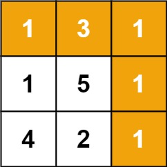
Input: grid = [[1,3,1],[1,5,1],[4,2,1]]
Output: 7
Explanation: Because the path 1 → 3 → 1 → 1 → 1 minimizes the sum.
Example 2:
Input: grid = [[1,2,3],[4,5,6]]
Output: 12
Constraints:
m == grid.lengthn == grid[i].length1 <= m, n <= 2000 <= grid[i][j] <= 200
Solution
Clarifying Questions
When you get asked this question in a real-life environment, it will often be ambiguous (especially at FAANG). Make sure to ask these questions in that case:
- What are the dimensions of the grid (number of rows and columns)? Can the grid be empty or have only one row/column?
- Are the numbers in the grid guaranteed to be non-negative as stated, or could there be negative numbers? What is the maximum possible value for a number in the grid?
- What should be returned if the grid is empty or if there's no path from the top-left to the bottom-right (e.g., if the grid has 0 rows or 0 columns)?
- Is it possible for the grid to contain duplicate numbers? If so, does this affect the path selection or the definition of a minimum sum path?
- Given that we can only move down or right, is it guaranteed that a path from the top-left to the bottom-right will always exist for any non-empty grid?
Brute Force Solution
Approach
To find the path with the smallest sum of numbers, we'll explore every single possible route from the start to the end. This means we consider all the different ways we can move, one step at a time, until we reach our destination.
Here's how the algorithm would work step-by-step:
- Start at the beginning of the grid.
- From your current spot, consider all the possible next moves (down or right).
- For each possible next move, calculate the sum of numbers along that particular path.
- Keep track of the smallest sum you've found so far.
- Repeat this process for every single path from the start to the end.
- Once you have explored all possible paths, the smallest sum you recorded will be the minimum path sum.
Code Implementation
def minimum_path_sum_brute_force(grid): rows_in_grid = len(grid) columns_in_grid = len(grid[0]) minimum_sum_found = float('inf') def explore_paths(current_row, current_column, current_path_sum): nonlocal minimum_sum_found # Add the value of the current cell to the path sum current_path_sum += grid[current_row][current_column] # Base case: if we've reached the bottom-right corner if current_row == rows_in_grid - 1 and current_column == columns_in_grid - 1: # Update the minimum sum if the current path is smaller minimum_sum_found = min(minimum_sum_found, current_path_sum) return # Explore moving down if current_row + 1 < rows_in_grid: explore_paths(current_row + 1, current_column, current_path_sum) # Explore moving right if current_column + 1 < columns_in_grid: explore_paths(current_row, current_column + 1, current_path_sum) # Start the exploration from the top-left corner explore_paths(0, 0, 0) return minimum_sum_foundBig(O) Analysis
Optimal Solution
Approach
This problem is about finding the cheapest way to get from the top-left corner of a grid to the bottom-right corner, only being able to move down or right. The clever strategy is to realize that the cheapest path to any particular spot in the grid must come from either the spot directly above it or the spot directly to its left. We can build up this knowledge from the start to the end.
Here's how the algorithm would work step-by-step:
- Imagine a grid where each cell has a cost associated with it.
- You start at the top-left cell.
- You want to reach the bottom-right cell by only moving one step down or one step right at a time.
- Your goal is to find a path where the sum of the costs of all the cells you visit is as small as possible.
- To solve this efficiently, think about the cost to reach any given cell.
- The cheapest way to get to a cell must be either by coming from the cell directly above it or from the cell directly to its left.
- So, for each cell, you calculate the minimum cost to reach it by adding the cell's own cost to the minimum cost of reaching either the cell above or the cell to the left.
- You apply this logic sequentially, starting from the initial cell and working your way across and down the grid.
- By the time you reach the bottom-right cell, you will have figured out the absolute minimum cost to get there.
Code Implementation
def minimum_path_sum(grid_of_costs):
    number_of_rows = len(grid_of_costs)
    number_of_columns = len(grid_of_costs[0])

    # Initialize a DP table to store minimum costs to reach each cell.
    minimum_costs_to_reach = [[0] * number_of_columns for _ in range(number_of_rows)]

    # The cost to reach the starting cell is its own value.
    minimum_costs_to_reach[0][0] = grid_of_costs[0][0]

    # Fill the first row: can only come from the left.
    for column_index in range(1, number_of_columns):
        minimum_costs_to_reach[0][column_index] = minimum_costs_to_reach[0][column_index - 1] + grid_of_costs[0][column_index]

    # Fill the first column: can only come from above.
    for row_index in range(1, number_of_rows):
        minimum_costs_to_reach[row_index][0] = minimum_costs_to_reach[row_index - 1][0] + grid_of_costs[row_index][0]

    # Compute minimum costs for the rest of the grid.
    for row_index in range(1, number_of_rows):
        for column_index in range(1, number_of_columns):
            # The minimum cost to reach this cell is its own cost plus the minimum of coming from above or from the left.
            cost_from_above = minimum_costs_to_reach[row_index - 1][column_index]
            cost_from_left = minimum_costs_to_reach[row_index][column_index - 1]
            minimum_costs_to_reach[row_index][column_index] = min(cost_from_above, cost_from_left) + grid_of_costs[row_index][column_index]

    # The bottom-right cell contains the overall minimum path sum.
return minimum_costs_to_reach[number_of_rows - 1][number_of_columns - 1]Big(O) Analysis
Edge Cases
| Case | How to Handle |
|---|---|
| Empty grid input | An empty grid should result in a sum of 0, or an error should be raised indicating invalid input. |
| Grid with zero rows or zero columns | A grid with no rows or no columns is invalid and should be handled with an appropriate error or a default return value like 0. |
| Grid with a single cell (1x1) | The path sum is simply the value of that single cell. |
| Grid with only one row or one column | The path is constrained to that single row or column, so the sum is the sum of all elements in that row/column. |
| All non-negative numbers are zero | The minimum path sum will be 0, as moving through zeros incurs no cost. |
| Very large grid dimensions | Dynamic programming solution should scale efficiently with time complexity O(m*n) and space complexity O(m*n) or O(min(m,n)) if optimized. |
| Integer overflow for sum calculation | Use a data type that can accommodate potentially large sums, such as a 64-bit integer, if the grid values and dimensions are large. |
| Non-negative numbers constraint violation (though problem states non-negative) | If negative numbers were allowed, the dynamic programming approach would still work correctly as it accounts for minimums. |