Number of Restricted Paths From First to Last Node

Medium

Asked by:

14 views

Topics:

GraphsDynamic Programming

There is an undirected weighted connected graph. You are given a positive integer n which denotes that the graph has n nodes labeled from 1 to n, and an array edges where each edges[i] = [u_i, v_i, weight_i] denotes that there is an edge between nodes u_i and v_i with weight equal to weight_i.

A path from node start to node end is a sequence of nodes [z₀, z₁,z₂, ..., z_k] such that z₀= start and z_k = end and there is an edge between z_i and z_i+1 where 0 <= i <= k-1.

The distance of a path is the sum of the weights on the edges of the path. Let distanceToLastNode(x) denote the shortest distance of a path between node n and node x. A restricted path is a path that also satisfies that distanceToLastNode(z_i) > distanceToLastNode(z_i+1) where 0 <= i <= k-1.

Return the number of restricted paths from node 1 to node n. Since that number may be too large, return it modulo 10⁹ + 7.

Example 1:

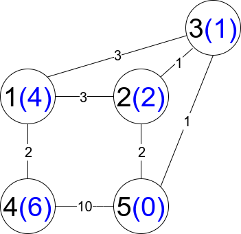
Input: n = 5, edges = [[1,2,3],[1,3,3],[2,3,1],[1,4,2],[5,2,2],[3,5,1],[5,4,10]]
Output: 3
Explanation: Each circle contains the node number in black and its distanceToLastNode value in blue. The three restricted paths are:
1) 1 --> 2 --> 5
2) 1 --> 2 --> 3 --> 5
3) 1 --> 3 --> 5

Example 2:

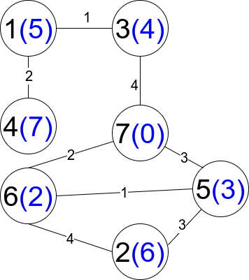
Input: n = 7, edges = [[1,3,1],[4,1,2],[7,3,4],[2,5,3],[5,6,1],[6,7,2],[7,5,3],[2,6,4]]
Output: 1
Explanation: Each circle contains the node number in black and its distanceToLastNode value in blue. The only restricted path is 1 --> 3 --> 7.

Constraints:

1 <= n <= 2 * 10⁴
n - 1 <= edges.length <= 4 * 10⁴
edges[i].length == 3
1 <= u_i, v_i <= n
u_i!= v_i
1 <= weight_i <= 10⁵
There is at most one edge between any two nodes.
There is at least one path between any two nodes.

Try coding it in LeetCode

Solution

Clarifying Questions

When you get asked this question in a real-life environment, it will often be ambiguous (especially at FAANG). Make sure to ask these questions in that case:

What is the maximum number of nodes (n) and edges (m) in the graph? This will help me understand the scale of the problem.
Can the edge weights (distances) be negative or zero?
If there are multiple shortest paths from the first node to the last node, should I count all restricted paths that utilize any of these shortest paths, or only those that utilize one specific shortest path?
If there is no path from the first node to the last node, or if there are no restricted paths, what should I return?
Are there any guarantees about the graph's connectivity? Specifically, is it guaranteed that there will always be at least one path from the first node to the last node?

Brute Force Solution

Approach

The brute force approach to finding restricted paths involves exploring every possible route from the starting point to the destination. We systematically check each path to see if it meets the 'restricted' criteria. This is like trying every road on a map until we find the ones that get us where we need to go and follow the rules.

Here's how the algorithm would work step-by-step:

Start at the first location.
Explore all possible paths you can take from your current location to a neighboring location.
For each neighboring location, again explore all possible paths from that location.
Continue exploring paths until you reach the final destination.
Every time you reach the final destination, check if the path you took is a 'restricted' path according to the problem's rules.
If the path is restricted, count it.
Repeat this process for all possible paths, making sure you don't get stuck in infinite loops by revisiting locations in ways that don't help you get closer to the destination.
The total number of restricted paths you counted is your answer.

Code Implementation

def number_of_restricted_paths(number_of_nodes, edges): 
    graph = [[] for _ in range(number_of_nodes + 1)]
    for start_node, end_node, weight in edges:
        graph[start_node].append((end_node, weight))
        graph[end_node].append((start_node, weight))

    distance = [float('inf')] * (number_of_nodes + 1)
    distance[number_of_nodes] = 0
    
    import heapq
    priority_queue = [(0, number_of_nodes)]

    while priority_queue:
        dist, node = heapq.heappop(priority_queue)

        if dist > distance[node]:
            continue

        for neighbor, weight in graph[node]:
            if distance[neighbor] > distance[node] + weight:
                distance[neighbor] = distance[node] + weight
                heapq.heappush(priority_queue, (distance[neighbor], neighbor))

    restricted_paths_count = 0
    
    def depth_first_search(current_node, visited):
        nonlocal restricted_paths_count

        if current_node == number_of_nodes:
            restricted_paths_count = (restricted_paths_count + 1) % (10**9 + 7)
            return

        for neighbor, _ in graph[current_node]:
            # Only explore neighbors that satisfy the restricted path condition
            if distance[current_node] > distance[neighbor]:
                depth_first_search(neighbor, visited | {neighbor})

    # Start the DFS from the first node
    depth_first_search(1, {1})

    return restricted_paths_count

Big(O) Analysis

Time Complexity

O(V!) – The brute force approach explores all possible paths from the start node to the end node in a graph with V vertices and E edges. In the worst-case scenario, every vertex could be connected to every other vertex, leading to a combinatorial explosion of paths to explore. Exploring all possible paths would be proportional to the number of permutations of vertices, resulting in a time complexity of O(V!), where V is the number of vertices. The 'restricted' path check doesn't fundamentally change this exhaustive path exploration cost.

Space Complexity

O(N) – The brute force approach, as described, explores all possible paths using a recursive depth-first search (DFS). The primary space contributor is the call stack used by the recursion, which, in the worst-case scenario, can reach a depth proportional to the number of nodes, N, in the graph as we explore long paths. We are also 'keeping track of visited locations' to avoid infinite loops, implying a boolean array of size N in the worst case. Therefore, the auxiliary space used is primarily determined by the recursion depth and visited node tracking, which can grow linearly with the number of nodes. This results in a space complexity of O(N).

Optimal Solution

Approach

The goal is to count the number of special routes from the beginning to the end of a map. We'll efficiently explore the map by focusing on paths where each step gets closer to the end, avoiding unnecessary backtracking.

Here's how the algorithm would work step-by-step:

First, figure out how far each location on the map is from the final destination. Use the distances between locations to compute this efficiently.
Once we know how far each place is from the end, we start exploring routes from the beginning.
At each location, only move to the next location if it's closer to the end than the current one.
Keep track of the number of routes that end up at the final destination.
To avoid repeating work, remember the number of routes from each location to the end. If you visit a location again, you can reuse the previously calculated route count.
Add up the number of routes to the destination, being careful to stay within the allowed range of values.

Code Implementation

import heapq

def countRestrictedPaths(number_of_nodes, edges):
    graph = [[] for _ in range(number_of_nodes + 1)]
    for node_a, node_b, weight in edges:
        graph[node_a].append((node_b, weight))
        graph[node_b].append((node_a, weight))

    distance_from_end = dijkstra(number_of_nodes, graph)
    
    number_of_paths = [0] * (number_of_nodes + 1)
    number_of_paths[number_of_nodes] = 1
    
    def dfs(current_node):
        if number_of_paths[current_node] != 0:
            return number_of_paths[current_node]
        
        paths = 0
        for neighbor, _ in graph[current_node]:
            # Visit only nodes closer to the end
            if distance_from_end[neighbor] < distance_from_end[current_node]:

                paths = (paths + dfs(neighbor)) % (10**9 + 7)
                
        number_of_paths[current_node] = paths
        return paths
    
    # Begin traversal from the start node
    return dfs(1)

def dijkstra(number_of_nodes, graph):
    distances = [float('inf')] * (number_of_nodes + 1)
    distances[number_of_nodes] = 0
    priority_queue = [(0, number_of_nodes)]
    
    while priority_queue:
        distance, current_node = heapq.heappop(priority_queue)
        
        if distance > distances[current_node]:
            continue
        
        for neighbor, weight in graph[current_node]:
            new_distance = distance + weight
            
            # Update shortest distance if a shorter path is found
            if new_distance < distances[neighbor]:

                distances[neighbor] = new_distance
                heapq.heappush(priority_queue, (new_distance, neighbor))
                
    return distances

Big(O) Analysis

Time Complexity

O(E log V) – The algorithm first computes the shortest distances from the last node to all other nodes using Dijkstra's algorithm, which takes O(E log V) time, where E is the number of edges and V is the number of vertices (nodes). Then, it performs a Depth-First Search (DFS) with memoization to count the number of restricted paths. The DFS visits each node at most once due to memoization. For each node, it iterates through its neighbors, which contributes a factor proportional to the degree of the node. In the worst case, the DFS visits all edges, but this is dominated by the initial Dijkstra's computation.

Space Complexity

O(N + E) – The algorithm uses a distance array of size N to store the distance from each node to the destination, where N is the number of nodes in the graph. Dijkstra's algorithm (implied by step 1) typically uses a priority queue, whose size can grow up to E, where E is the number of edges. The algorithm also utilizes memoization (step 5), storing the number of paths from each node to the destination, resulting in an array of size N. Therefore, the auxiliary space complexity is O(N + E + N), which simplifies to O(N + E).

Edge Cases

Case	How to Handle
Empty graph (no edges)	Return 0 if the graph has no edges as there are no paths.
Single node graph	If the graph consists of a single node, the path count is 1 (the node itself).
Graph with no path between start and end nodes	The algorithm should return 0 when there is no path from the first to the last node by resulting in an empty priority queue after Dijkstra's algorithm.
Graph with cycles	Dijkstra's algorithm and dynamic programming inherently handle cycles as we only consider nodes with a smaller distance to the target node preventing infinite loops.
Large graph (many nodes and edges)	The algorithm needs to be efficient, using Dijkstra's algorithm with a priority queue for performance, and dynamic programming to avoid recomputation.
Weights causing integer overflow during distance calculation	Use a larger data type like long to store distances to prevent integer overflow during distance calculations.
Graph where all edges have the same weight	Dijkstra's still works correctly but the priority queue might degrade in performance compared to graphs with diverse edge weights.
The last node is unreachable during distance calculation	If the distance to the last node is infinity after Dijkstra, it means there are no paths, return 0.

Empty graph (no edges)

How to Handle:

Return 0 if the graph has no edges as there are no paths.

Single node graph

How to Handle:

If the graph consists of a single node, the path count is 1 (the node itself).

Graph with no path between start and end nodes

How to Handle:

The algorithm should return 0 when there is no path from the first to the last node by resulting in an empty priority queue after Dijkstra's algorithm.

Graph with cycles

How to Handle:

Dijkstra's algorithm and dynamic programming inherently handle cycles as we only consider nodes with a smaller distance to the target node preventing infinite loops.

Large graph (many nodes and edges)

How to Handle:

The algorithm needs to be efficient, using Dijkstra's algorithm with a priority queue for performance, and dynamic programming to avoid recomputation.

Weights causing integer overflow during distance calculation

How to Handle:

Use a larger data type like long to store distances to prevent integer overflow during distance calculations.

Graph where all edges have the same weight

How to Handle:

Dijkstra's still works correctly but the priority queue might degrade in performance compared to graphs with diverse edge weights.

The last node is unreachable during distance calculation

How to Handle:

If the distance to the last node is infinity after Dijkstra, it means there are no paths, return 0.