
Shortest Path Visiting All Nodes
Hard



You have an undirected, connected graph of n nodes labeled from 0 to n - 1. You are given an array graph where graph[i] is a list of all the nodes connected with node i by an edge.
Return the length of the shortest path that visits every node. You may start and stop at any node, you may revisit nodes multiple times, and you may reuse edges.
Example 1:
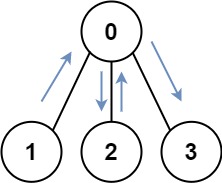
Input: graph = [[1,2,3],[0],[0],[0]]
Output: 4
Explanation: One possible path is [1,0,2,0,3]
Example 2:
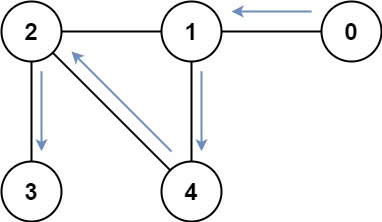
Input: graph = [[1],[0,2,4],[1,3,4],[2],[1,2]]
Output: 4
Explanation: One possible path is [0,1,4,2,3]
Constraints:
n == graph.length1 <= n <= 120 <= graph[i].length < ngraph[i]does not containi.- If
graph[a]containsb, thengraph[b]containsa. - The input graph is always connected.

Solution
Clarifying Questions
When you get asked this question in a real-life environment, it will often be ambiguous (especially at FAANG). Make sure to ask these questions in that case:
- What is the format of the input? Is it a list of lists representing an adjacency matrix or an adjacency list, or is it something else?
- How many nodes are in the graph (what's the maximum value of 'n')?
- Are the graph edges directed or undirected?
- Is the graph guaranteed to be connected?
- If it is not possible to visit all nodes, what value should I return?
Brute Force Solution
Approach
The goal is to find the shortest route that visits every location on a map. The brute force method explores every possible path to find the shortest one. It's like trying every single road combination until we find the absolute shortest way to visit all the locations.
Here's how the algorithm would work step-by-step:
- Start at one of the locations.
- From that location, explore every possible next location to visit.
- Continue this process, exploring all possible paths from each new location, making sure not to revisit a location until all other locations have been visited.
- Keep track of the length of each path that visits all locations.
- Compare the lengths of all the paths that visit all locations.
- The shortest path found is the answer.
Code Implementation
def shortest_path_visiting_all_nodes_brute_force(graph):
    number_of_nodes = len(graph)
    shortest_path_length = float('inf')

    def solve(current_node, visited_nodes, current_path_length, current_path):
        nonlocal shortest_path_length

        # All nodes visited, potentially update shortest path
        if visited_nodes == (1 << number_of_nodes) - 1:

            shortest_path_length = min(shortest_path_length, current_path_length)
            return

        # Optimization: If current path is already longer than shortest, stop
        if current_path_length >= shortest_path_length:
            return

        for next_node in graph[current_node]:
            # Avoid cycles when other nodes have not yet been visited
            if (visited_nodes & (1 << next_node)) == 0:
                solve(next_node, visited_nodes | (1 << next_node), current_path_length + 1, current_path + [next_node])
            else:
                solve(next_node, visited_nodes, current_path_length + 1, current_path + [next_node])

    # Iterate through all starting nodes to find optimal solution
    for start_node in range(number_of_nodes):

        # Ensures every node is tried as a start
        solve(start_node, 1 << start_node, 0, [start_node])

    # Must return an integer representing path length
return shortest_path_lengthBig(O) Analysis
Optimal Solution
Approach
The core idea is to explore possible paths while remembering which nodes we've already visited. Since we want the shortest path, we cleverly prioritize paths that explore new nodes quickly, avoiding redundant revisits of the same sets of nodes.
Here's how the algorithm would work step-by-step:
- Imagine each node in the graph as a city you need to visit.
- Start by considering every city as a possible starting point.
- Keep track of which cities you've visited along each path.
- As you explore paths, remember the minimum cost or length it takes to visit a specific set of cities.
- When you come across the same set of visited cities at a higher cost, ignore that path, because you already know a better way to reach those cities.
- Keep exploring until you find the shortest path that allows you to visit every city.
- The key is to remember the best way to visit any combination of cities, this avoids getting stuck exploring inefficient paths.
Code Implementation
from collections import deque

def shortest_path_visiting_all_nodes(graph):
    number_of_nodes = len(graph)
    all_nodes_visited = (1 << number_of_nodes) - 1

    queue = deque()
    # Initialize the queue with each node as a starting point.
    for start_node in range(number_of_nodes):
        queue.append((start_node, 1 << start_node, 0))

    # Keep track of visited states (node, mask) with shortest path length.
    visited = set()

    while queue:
        current_node, current_mask, path_length = queue.popleft()

        # If we've visited all nodes, return the path length.
        if current_mask == all_nodes_visited:
            return path_length

        # Skip if this state has been visited with a shorter path.
        if (current_node, current_mask) in visited:
            continue

        visited.add((current_node, current_mask))

        # Explore neighbors of the current node.
        for neighbor in graph[current_node]:
            new_mask = current_mask | (1 << neighbor)
            queue.append((neighbor, new_mask, path_length + 1))

return 0Big(O) Analysis
Edge Cases
| Case | How to Handle |
|---|---|
| Null or empty graph (graph is None or has no nodes) | Return 0 if the graph is empty, as there are no nodes to visit; otherwise, if graph is not None but has no nodes (an empty list), return 0. |
| Graph with only one node | Return 0, since all nodes (which is just one) are already visited. |
| Graph with two nodes and no edges | Return 1, as we must traverse between the two disconnected nodes. |
| Complete graph (every node connected to every other node) | The algorithm should still work correctly, potentially finding an optimal path quickly, and the solution's time complexity should not change drastically. |
| Disconnected graph (not all nodes are reachable from any starting node) | If the mask is never fully set to indicate that all nodes have been visited, then the algorithm will loop indefinitely or exceed time limits, so the solution must return -1 if a full visit is not possible within a reasonable number of steps, or avoid disconnected nodes with pre-checks. |
| Graph with a single long path (essentially a linked list) | The BFS might take longer to explore all possible paths, potentially impacting performance, so a dynamic programming approach would be better if we expect this type of graphs regularly. |
| Cyclic graph | The BFS approach with a visited set can handle cycles without infinite loops, as the state (node and mask) will prevent re-visiting the same node with the same visited node set. |
| Graph with large number of nodes | The BFS approach using bitmasking for visited states can lead to large queue sizes and memory consumption (O(2^N * N)), so we should consider alternative algorithms or approximations if N is very large (e.g., > 20), and document the complexity constraints clearly. |